Day 6 of the #30DayMapChallenge - Blue

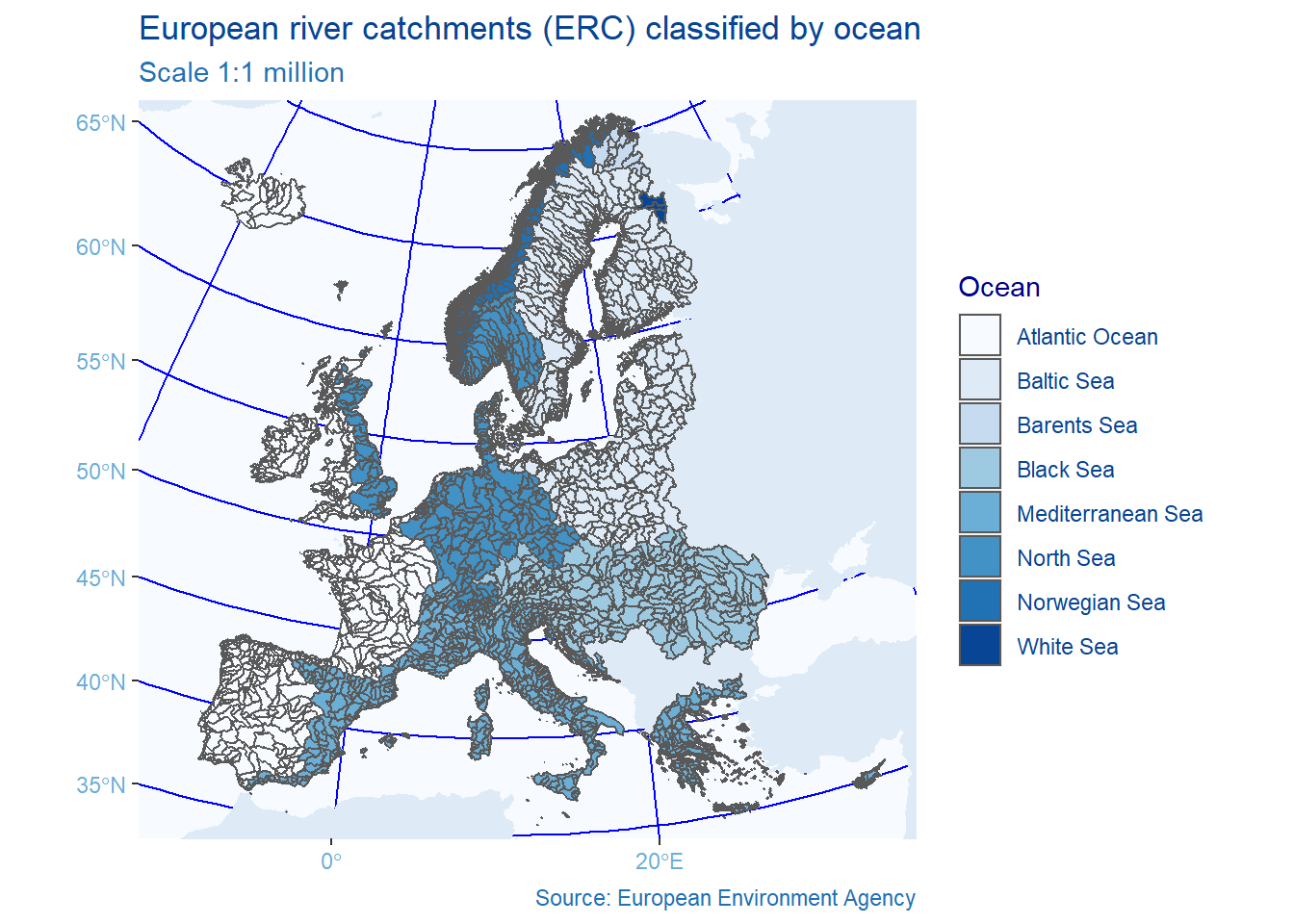
I plotted the European river catchments changing the default settings in ggplot2 to different scales of blue (e.g. background, grids, etc.).

Load packages:

  library(sf)
  library(tidyverse)
  library(rworldmap)
  library(rworldxtra)

1. Download the European river catchments from the European Environment Agency:

  dir.create("Rdata") # create a new folder (i.e. Rdata)
  
  River_URL <- "https://www.eea.europa.eu/data-and-maps/data/european-river-catchments-1/zipped-shapefile-vector-polygon/zipped-shapefile-vector-polygon/at_download/file.zip"
  download.file(River_URL, destfile = "Rdata/River.zip")
  unzip(zipfile = "Rdata/River.zip", exdir   = "Rdata/River")
  River <- read_sf("Rdata/River/ERC110108v2.shp")

2. Load World map {rworldmap}, and transform its coordinate system to the CRS of “River” (sf::st_transform):

World <- rworldmap::getMap(resolution = "high") %>% 
  st_as_sf() %>%
    st_transform(crs = st_crs(River))

unlink("Rdata", recursive = TRUE) # Delate Rdata

3. Plot results in blue:

  ggplot() +
    geom_sf(data = World, col = "#DEEBF7", fill = "#DEEBF7") +
    geom_sf(data = River, aes(fill = OCEAN_1)) +
    scale_fill_brewer(name = "Ocean", palette = "Blues") +
    coord_sf(xlim = c(2500000, 6500000), ylim = c(1500000, 5300000)) +
    labs(title = "European river catchments (ERC) classified by ocean",
         subtitle = "Scale 1:1 million",
         caption = "Source: European Environment Agency", color = "blue") +
    theme(axis.text = element_text(colour = "#6BAED6"),
          plot.title = element_text(colour = "#084594"),
          plot.subtitle = element_text(colour = "#2171B5"),
          plot.caption = element_text(colour = "#2171B5"),
          legend.title = element_text(color = "darkblue"),
          legend.text = element_text(color = "#084594"),
          panel.background = element_rect(fill = "#F7FBFF"),
          panel.grid.major = element_line(colour = "blue"))