Day 25 of the #30DayMapChallenge - Climate

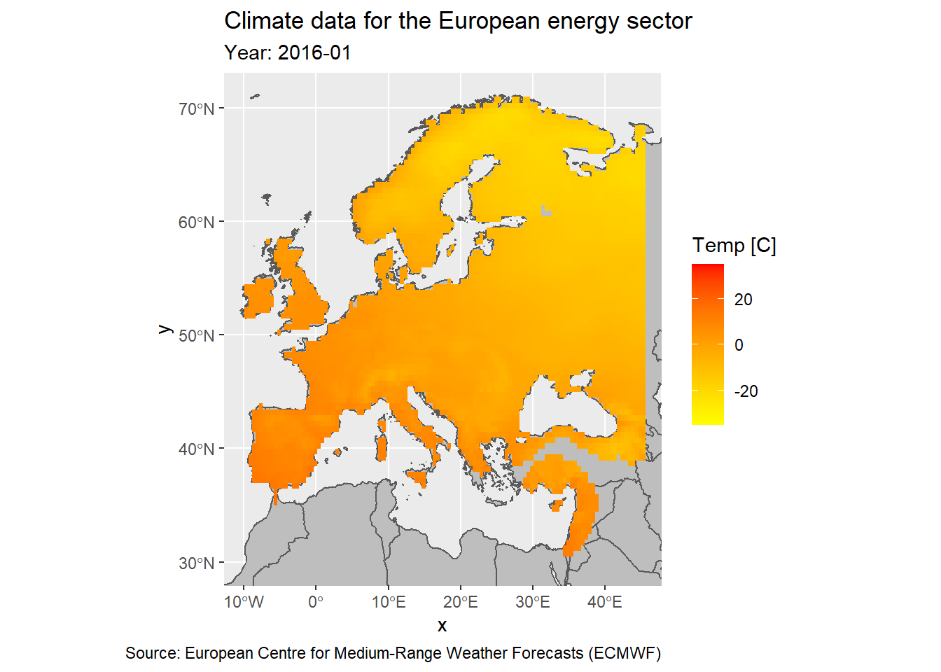
Plot the temperature of the air at about 2m above the surface (i.e. monthly averages).

Packages we are going to use:

  library(raster)
  library(animation)
  library(ncdf4)
  library(sf)
  library(ggplot2)
  library(rworldmap)
  library(rworldxtra)

Firstly, I have downloaded the monthly average temperatures from ECMWF. You may need to register for the Climate Data Store - CDS, but it is free and there are plenty of interesting data sets!. I have download the Climate data for the European energy sector from 1979 to 2016 derived from ERA-Interim:

• Variable: Air temperature
• Time aggregation: month average
• Vertical level: 2 m
• Bias correction: Normal distribution adjustment
• Format: Zip file

Then, we need to load the data into R. I have created a vector (Years) with dates from Feb. 1979 to Dec. 2016, we will use it for adding the date (year, month) to the rasters of temperature distribution (resolution 0.5° x 0.5°).

# Vector with years and months
  Years <- seq(as.Date("1979/01/01"), as.Date("2016/12/01"), by = "month")
  Years <- format(Years, "%Y-%m")
  
# Load the temperatures as a list with raster layers 
  Temp_m <- list()
  for (i in seq_along(Years)) {
    Temp_m[i] <- raster("H_ERAI_ECMW_T159_TA-_0002m_Euro_22W27N_45E72N_050d_IN_TIM_19790101_20161231_01m_NA-_nbc_org_NA_NA-.nc", i)
  }
  Temp_m <- brick(Temp_m)

# Convert to a data frame with rasters
  raster_df <- as.data.frame(Temp_m, xy = TRUE)

We also need to load the world map for plotting the temperatures, in this case I have used the R package rworldmap.

World <- rworldmap::getMap(resolution = "high") %>% 
  st_as_sf() # Convert to an sf object

Finally, I have created an auxiliary function (Steps(i)) for plotting the monthly average temperatures. We will use it for plotting the temperatures by month (i.e. Jan. 2016) and for making animations (i.e. monthly average temperatures in 2016). The function (Steps(i)) will plot the temperature in the month i = 1, 2, …, 456, where 1 = 1979-01; 2 = 1979-02, …, and 456 = 2016-12.

Steps <- function(i) {
    p <- ggplot() +
      geom_sf(data = World, fill = "grey") +
      geom_raster(data = raster_df,
                  aes(x = x, y = y, fill = raster_df[[i+2]])) +
      scale_fill_gradient("Temp [C]",
                          low = 'yellow', high = 'red',
                          na.value = NA,
                          limits = c(-35, 35)) +
      coord_sf(xlim = c(-10, 45), ylim = c(30, 71)) +
      labs(title = "Climate data for the European energy sector",
           subtitle = paste("Year:", Years[i]),
           caption = "Source: European Centre for Medium-Range Weather Forecasts (ECMWF)")
    print(p) 
  }

Average temperatures in Jan. 2016.

Steps(445)

For the animation I loop the function Steps from 445 (Jan. 2016) to 456 (Dic. 2016), and save the result as .gif:

animation::saveGIF(for(i in 445:456) Steps(i), 
                     interval = 0.2,
                     movie.name = "Day25_Temp_AV_month_2m_2016.gif")