Day 3 of the #30DayMapChallenge - Polygons

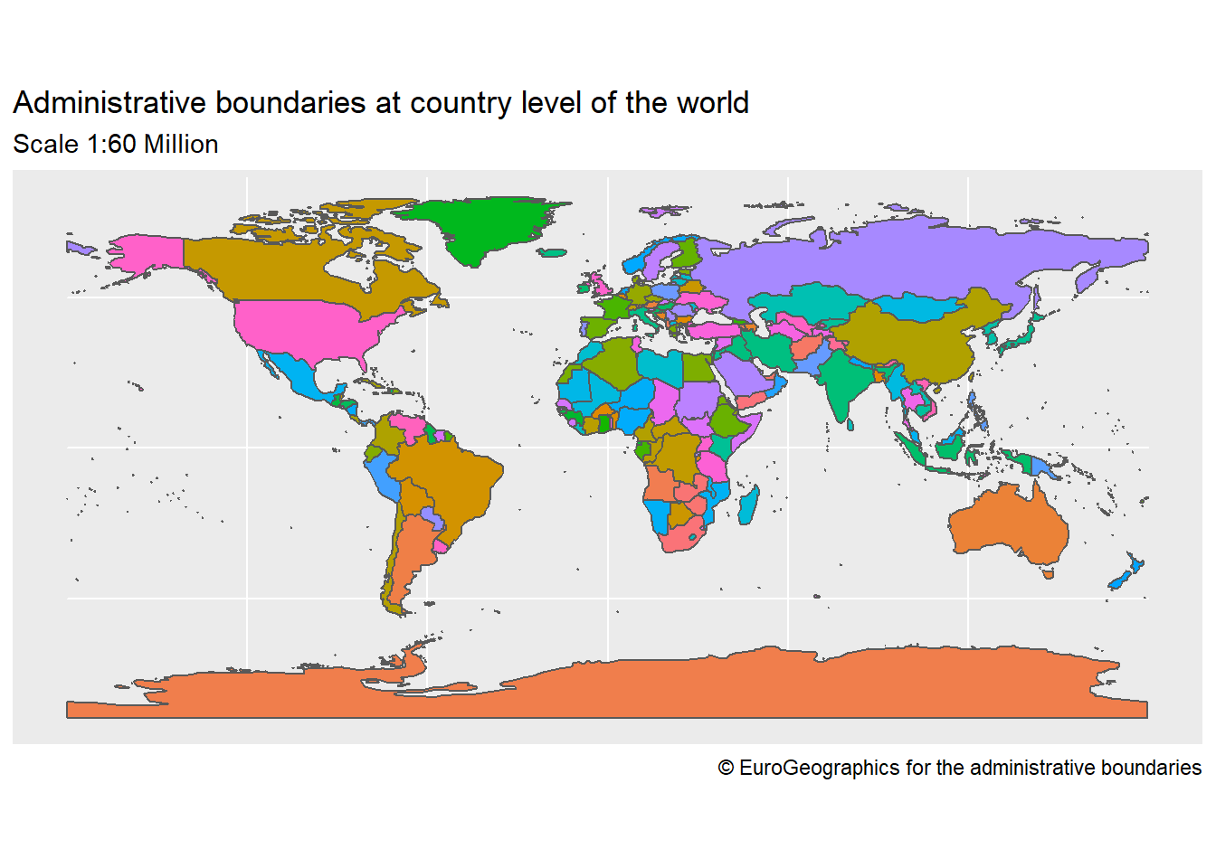
I plotted a wold map (scale 1:60 Million) with color varying by country.

1. Download the data from Eurostat, where there are geographic data of:

   • Administrative units – statistical units

   • Population distribution – demography

   • Transport networks

   • Land cover

   • Elevation – DEM

Packages we are going to use:

  library(sf)
  library(tidyverse)

  World_URL <- "https://ec.europa.eu/eurostat/cache/GISCO/distribution/v2/countries/download/ref-countries-2016-60m.shp.zip"
  dir.create("Rdata")
  download.file(World_URL, destfile = "Rdata/World.zip")
  unzip(zipfile = "Rdata/World.zip", exdir   = "Rdata/World")
  unzip(zipfile = "Rdata/World/CNTR_RG_60M_2016_4326.shp.zip",
        exdir   = "Rdata/World_SHP")
  World <- read_sf("Rdata/World_SHP/CNTR_RG_60M_2016_4326.shp")
  unlink("Rdata", recursive = TRUE)

2. Plot the results with fill = CNTR_ID.

  ggplot() +
    geom_sf(data = World, aes(fill = CNTR_ID)) +
    labs(title = "Administrative boundaries at country level of the world",
         subtitle = "Scale 1:60 Million",
         caption = "© EuroGeographics for the administrative boundaries") +
    guides(fill = FALSE)