Data visualization in R: line charts (cont)
In the previous post we saw how to plot line charts in R using the package ggplot2. I will continue with this topic and we will learn additional features that may be useful for data visualization, in particular:
- Create our own customize ggplot2 theme.
- Combine on the same plot several ggplot objects with patchwork.
- Export ggplot objects.
We will use the following libraries:
library(danstat)
library(furrr)
library(tidyverse)
library(readr)
library(dint)
library(patchwork)
library(forcats)
Create our own customize plot theme
The theme is the part of the code where we define the non-data elements of our plot. In this sense, it is the part where we specify, for example, the fonts or backgrounds of the figure but not how the data are rendered. It is therefore called after defining how the data shall be plotted (e.g. geom_line) and it takes the form of theme(…). There are already nine predefined themes (e.g. theme_bw, theme_classic, …; see figure) which are optimized for data visualization (for more details please see the chapter 18 of ggplot2: Elegant Graphics for Data Analysis.
df <- tribble(~x, ~y,
              1, 1,
              2, 2)
p <- ggplot(df, aes(x = x, y = y)) + geom_line(col = "red") + geom_point(col = 4)

p1 <- p + theme_gray() + labs(title = "theme_gray - default")
p2 <- p + theme_bw() + labs(title = "theme_bw")
p3 <- p + theme_linedraw() + labs(title = "theme_linedraw")
p4 <- p + theme_light() + labs(title = "theme_light")
p5 <- p + theme_dark() + labs(title = "theme_dark")
p6 <- p + theme_minimal() + labs(title = "theme_minimal")
p7 <- p + theme_classic() + labs(title = "theme_classic")
p8 <- p + theme_void() + labs(title = "theme_void")
p9 <- p + theme_test() + labs(title = "theme_test")

p1 + p2 + p3 + p4 + p5 + p6 + p7 + p8 + p9
The package ggthemes provides additional themes. However, even with all these predefined themes we may not find the one which matchs our needs and we would need to modify individual components. We can do that with the function theme and thus create our own customized theme.
my_theme <- function() {
  theme_bw() +
    theme(
      # Title and captions
      plot.title = element_text(size = 14, colour = "darkblue", face = "bold"),
      plot.caption = element_text(size = 9, colour = "grey25"),
      # Labels
      axis.title = element_text(size = 11, face = "bold"),
      axis.text = element_text(size = 9),
      # Background colour
      plot.background = element_rect(fill = "linen", colour = NA),
      # Legend
      legend.title = element_text(size = 9, face = "bold"),
      legend.background = element_rect(fill = "linen", color = NA),
      legend.key = element_rect(fill = "linen"),
      # Facets
      strip.text = element_text(size = 12, color = "white", face = "bold.italic"),
      strip.background = element_rect(color = "black", fill = "#FC4E07", linetype = "solid")
    )
}

p + my_theme() + labs(title = "my_theme",
                      caption = "my_theme")
Load data
Now that we have seen how to change the aesthetic of our plot (the non-data parts) we will use our own theme with our data, and we will plot the population change of the top 10 immigration groups in Denmark from 2008. We will need to download from Statistic Denmark the population at the first day of the quarter by region, ancestry, and country of origin (Table: FOLK1C). If you want to see in detail the process you can read my previous post Get free data from Statistic Denmark, and the data cleaning process in Data visualization in R: line charts.
id_table <- "FOLK1C"
var_pop  <- get_table_metadata(table_id = id_table, variables_only = TRUE)

# loop by quarter for getting the data
steps <- function(quarter){
  var_values <- list(id_region, id_ancestry, id_citizen, quarter)
  var_input <- purrr::map2(.x = var_codes,
                           .y = var_values,
                           .f = ~list(code = .x, values = .y))
  get_data(id_table, variables = var_input)
}

# Codes for var_input
var_codes <- c("OMRÅDE", "HERKOMST", "IELAND", "Tid")

# Values for var_input
## Region: All Denmark
id_region <- "000"
## Ancestry (Immigrants and Descendant)
id_ancestry <- c(4, 3)
## Country of origin (remove total)
id_citizen <- as.numeric(var_pop$values[[5]]$id)
id_citizen <- id_citizen[id_citizen > 0]
## Quarters
id_quarter <- var_pop$values[[6]]$id
# Parallel process with {future}
plan(multisession)
pop_migr <- id_quarter %>% future_map(steps)
pop_migr <- bind_rows(pop_migr)
plan("default")

# Clean column names and format some data

pop_migr <- pop_migr %>%
  # translate columns names into English
  rename(region = OMRÅDE,
         ancestry = HERKOMST,
         origin = IELAND,
         date = TID,
         pop = INDHOLD) %>%
  # Transform date
  mutate(date = gsub("Q", "", date),
         date = as_date_yq(as.integer(date)),
         date = first_of_quarter(date)) %>%
  # Total Immigrants and Descendants by region, date, and country of origin
  pivot_wider(c(region, origin, date), names_from = ancestry, values_from = pop) %>%
  mutate(Total = Immigrants + Descendant) %>%
  pivot_longer(cols = c(Immigrants, Descendant, Total),
               values_to = "pop",
               names_to = "ancestry")

pop_migr
## # A tibble: 36,972 x 5
## region origin date ancestry pop
## <chr> <chr> <date> <chr> <dbl>
## 1 All Denmark Denmark 2008-01-01 Immigrants 0
## 2 All Denmark Denmark 2008-01-01 Descendant 0
## 3 All Denmark Denmark 2008-01-01 Total 0
## 4 All Denmark Albania 2008-01-01 Immigrants 213
## 5 All Denmark Albania 2008-01-01 Descendant 33
## 6 All Denmark Albania 2008-01-01 Total 246
## 7 All Denmark Andorra 2008-01-01 Immigrants 0
## 8 All Denmark Andorra 2008-01-01 Descendant 0
## 9 All Denmark Andorra 2008-01-01 Total 0
## 10 All Denmark Belgium 2008-01-01 Immigrants 850
## # ... with 36,962 more rowsDetect the top 10 immigration groups in 2020
We got the foreign population by country of origin from 2008 to 2020. Now, we need to detect the top 10 countries of origin in terms of the total immigrant population (i.e. Total = Immigrants + Descendant) in 2020. Note that the data are in the long format (one row for each measurement) but we are only interested in the total population. Therefore, we also need to subset the data frame by ancestry = Total and not only by date. This is done by the function filter and defining two arguments (date and ancestry). Then, we would need to order the data base on the total population and select the 10 first rows. However, there is already a function for doing that (slice_max).
top10_countries <- pop_migr %>%
  filter(date == as.Date("2020-10-01"),
         ancestry == "Total") %>%
  slice_max(pop, n = 10)

top10_countries
## # A tibble: 10 x 5
## region origin date ancestry pop
## <chr> <chr> <date> <chr> <dbl>
## 1 All Denmark Turkey 2020-10-01 Total 64492
## 2 All Denmark Poland 2020-10-01 Total 48664
## 3 All Denmark Syria 2020-10-01 Total 43679
## 4 All Denmark Germany 2020-10-01 Total 34733
## 5 All Denmark Romania 2020-10-01 Total 34459
## 6 All Denmark Iraq 2020-10-01 Total 33694
## 7 All Denmark Lebanon 2020-10-01 Total 27539
## 8 All Denmark Pakistan 2020-10-01 Total 26151
## 9 All Denmark Bosnia and Herzegovina 2020-10-01 Total 23258
## 10 All Denmark Iran 2020-10-01 Total 22043We can see the most representative countries of origin within the Danish immigrant population in 2020. Now, we are going to evaluate the evolution of these groups over the last years (from 2008 that is the first year we have data from Statistic Denmark). Therefore, we need to subset our data frame (pop_migr) to get only the data from the top 10 countries of origin. As we saw before we can do that using the function filter. However, in this case we are not interested only in one value (e.g. ancestry == “Total”) but in the identification of all the elements (i.e. origin) within a vector (top10_countries$origin) and we need to use the operator %in%.
pop_migr_top10 <- pop_migr%>%
  filter(origin %in% top10_countries$origin) %>%
  # Wide format
  pivot_wider(c(origin, date), names_from = ancestry, values_from = pop) %>%
  # Reorder origin factors by Total population in 2020-Q3
  mutate(origin = factor(origin),
         origin = fct_reorder2(origin, date, Total))

pop_migr_top10
## # A tibble: 520 x 5
## origin date Immigrants Descendant Total
## <fct> <date> <dbl> <dbl> <dbl>
## 1 Bosnia and Herzegovina 2008-01-01 17987 3859 21846
## 2 Poland 2008-01-01 18506 2546 21052
## 3 Romania 2008-01-01 3277 399 3676
## 4 Turkey 2008-01-01 31433 25696 57129
## 5 Germany 2008-01-01 25827 2462 28289
## 6 Iraq 2008-01-01 21181 7232 28413
## 7 Iran 2008-01-01 11853 2911 14764
## 8 Lebanon 2008-01-01 12034 11252 23286
## 9 Pakistan 2008-01-01 10617 8861 19478
## 10 Syria 2008-01-01 1778 1546 3324
## # ... with 510 more rowsPlots
Plot the total population change.
p_tot <- pop_migr_top10 %>%
  ggplot() +
  geom_line(aes(x = date, y = Total/1000, colour = origin), size = 0.7) +
  my_theme() +
  labs(#title = "Immigrants and descendants in Denmark",
       subtitle = "Top 10 countries of origin in 2020",
       y = "Pop [x1000]",
       x = "") +
  scale_color_brewer(name = "Country of\norigin", palette = "Paired")

p_tot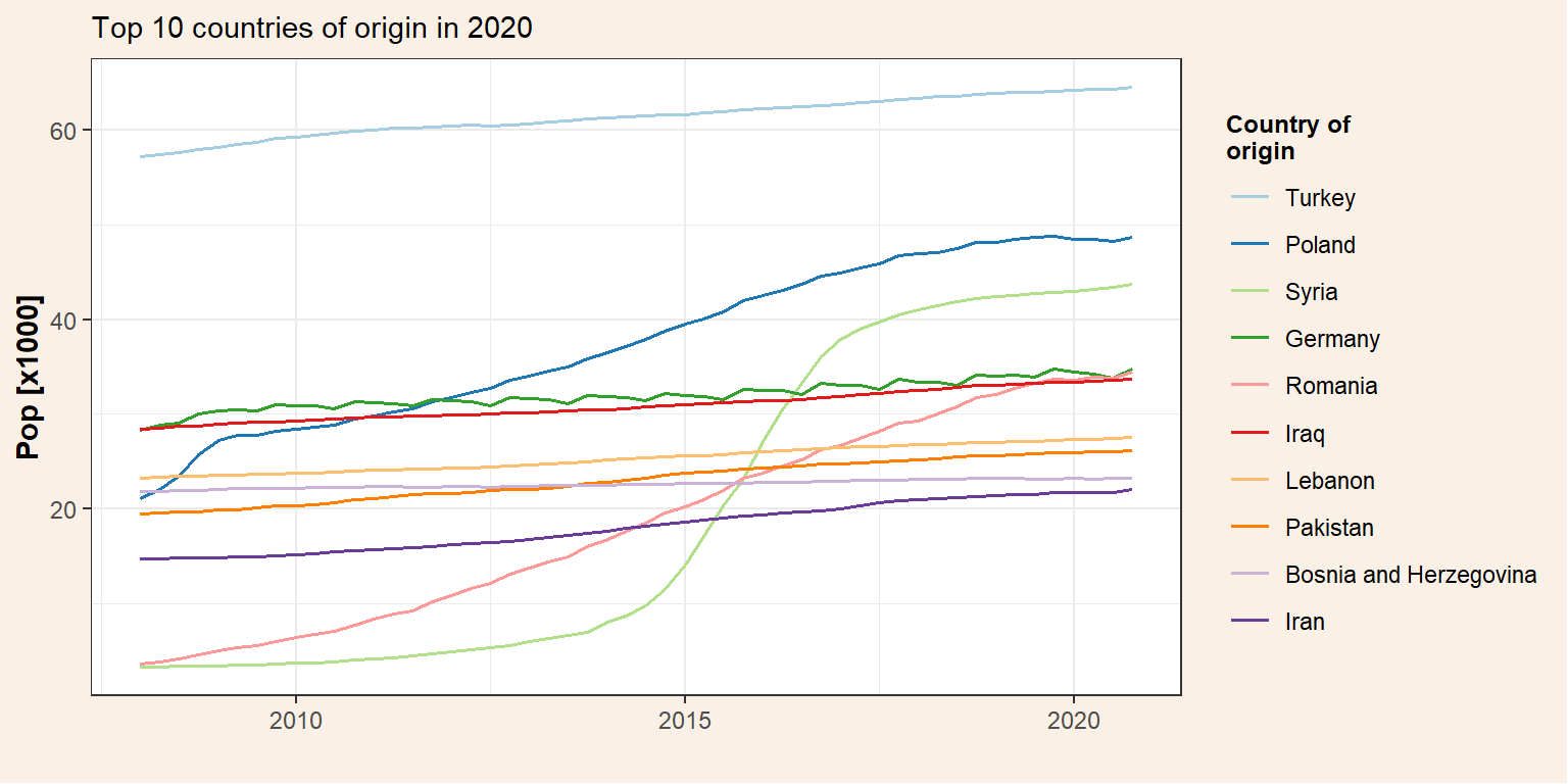
Plot the evolution of immigrants and their descendants independently.
p_id <- pop_migr_top10 %>%
  select(-Total) %>%
  pivot_longer(cols = c(Immigrants, Descendant), names_to = "ancestry", values_to = "pop") %>%
  mutate(ancestry = factor(ancestry, levels = c("Immigrants","Descendant"))) %>%
  ggplot() +
  geom_line(aes(x = date, y = pop/1000, colour = origin), size = 0.7) +
  facet_grid(~ancestry) +
  my_theme() +
  labs(subtitle = "Divided by ancestry",
       y = "Pop [x1000]",
       x = "") +
  scale_color_brewer(name = "Country of\norigin", palette = "Paired")

p_id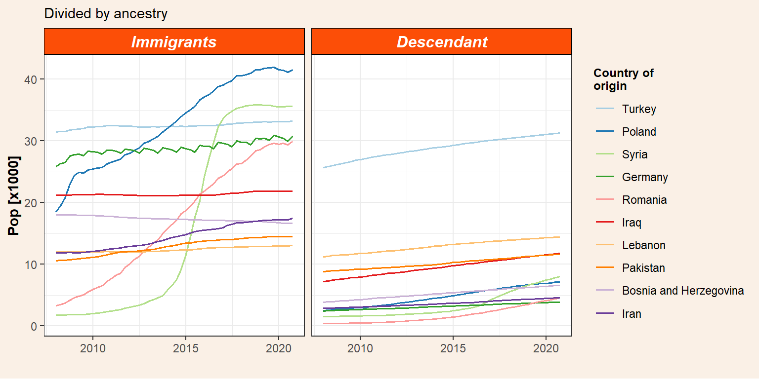
Now that we have two ggplot objects we can plot them together. There are several ways to do that but I found the package patchwork the simplest one. It is really intuitive and use the operators +, |, and / for adding plots together. In this sense, + adds the figures in row order trying to keep a grid square while | places the plots beside each other and / stacks them. Therefore, if we want to plot together our immigration figures with the total population (p_tot) on top we use the / operator.
p_tot / p_id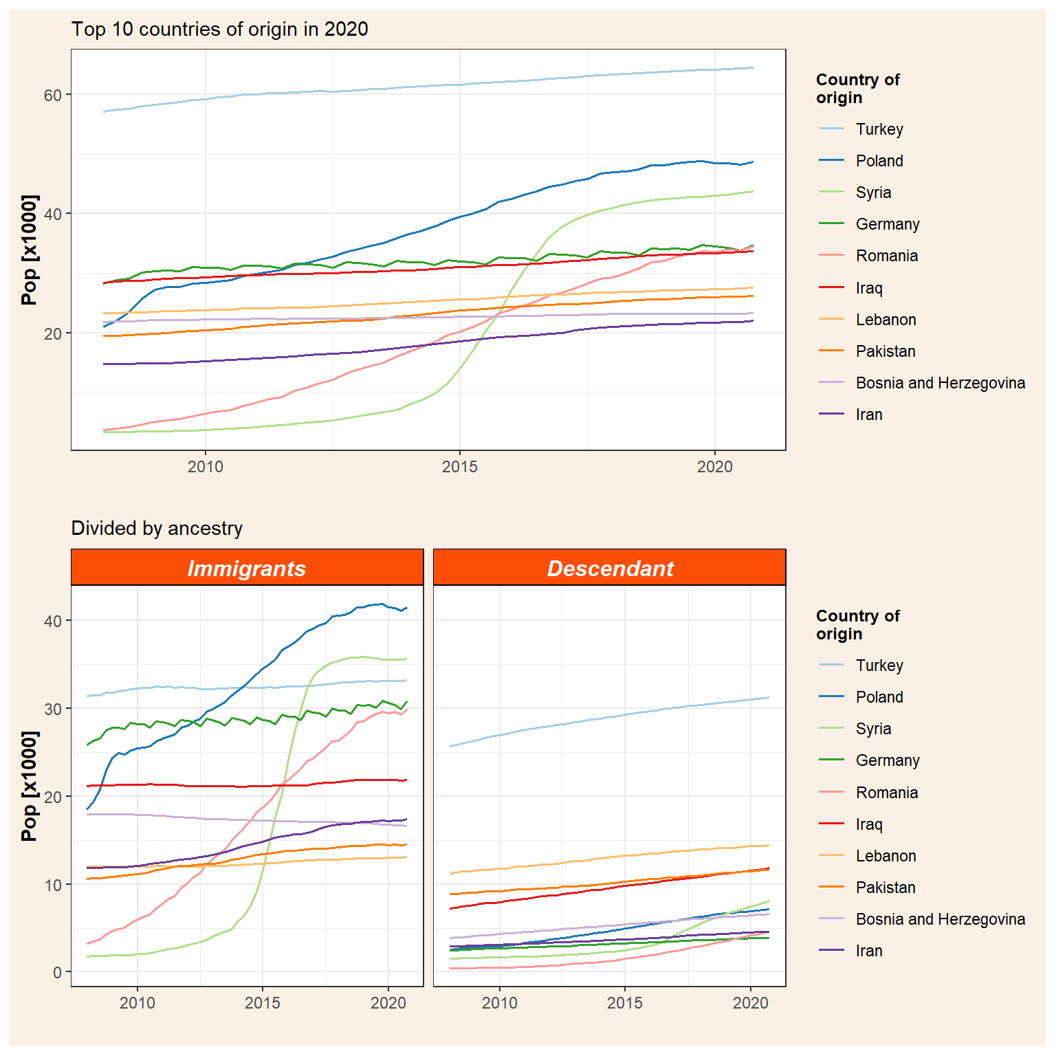
Note that both figures share the same legend and thus we can combine them by adding a plot_layout. We can also add titles, captions, and tags with plot_annotation. Furthermore, in plot_annotation there is an argument where we can control the theme as we saw before and therefore we can, for example, change the colour of the outline border (from white to the same colour of our background) or the size and colour of the title and captions.
p_top10 <- p_tot / p_id +
  plot_layout(guides = "collect") +
  plot_annotation(title = "Immigrants and descendants in Denmark",
                  caption = "Data source: Statistics Denmark\nAuthor: J. Elio (@Elio_Javi), C. Keßler, H.S. Hansen. Aalborg University, Department of Planning",
                  tag_levels = "A",
                  theme = theme(plot.background = element_rect(color  = NA, fill = "linen"),
                                plot.title = element_text(size = 14, colour = "darkblue", face = "bold"),
                                plot.caption = element_text(size = 9, colour = "grey25")))
Finally, ggsave can be used to export a plot. We’d need to specify the ggplot object we would like to save (by default the last one) and the format (e.g. .pdf, .jpeg, .tiff, .png, etc.) and the size, file name, …
ggsave(plot = p_top10,
       filename = "featured.png",
       width = 20,
       height = 20,
       units = "cm")
knitr::include_graphics("featured.png")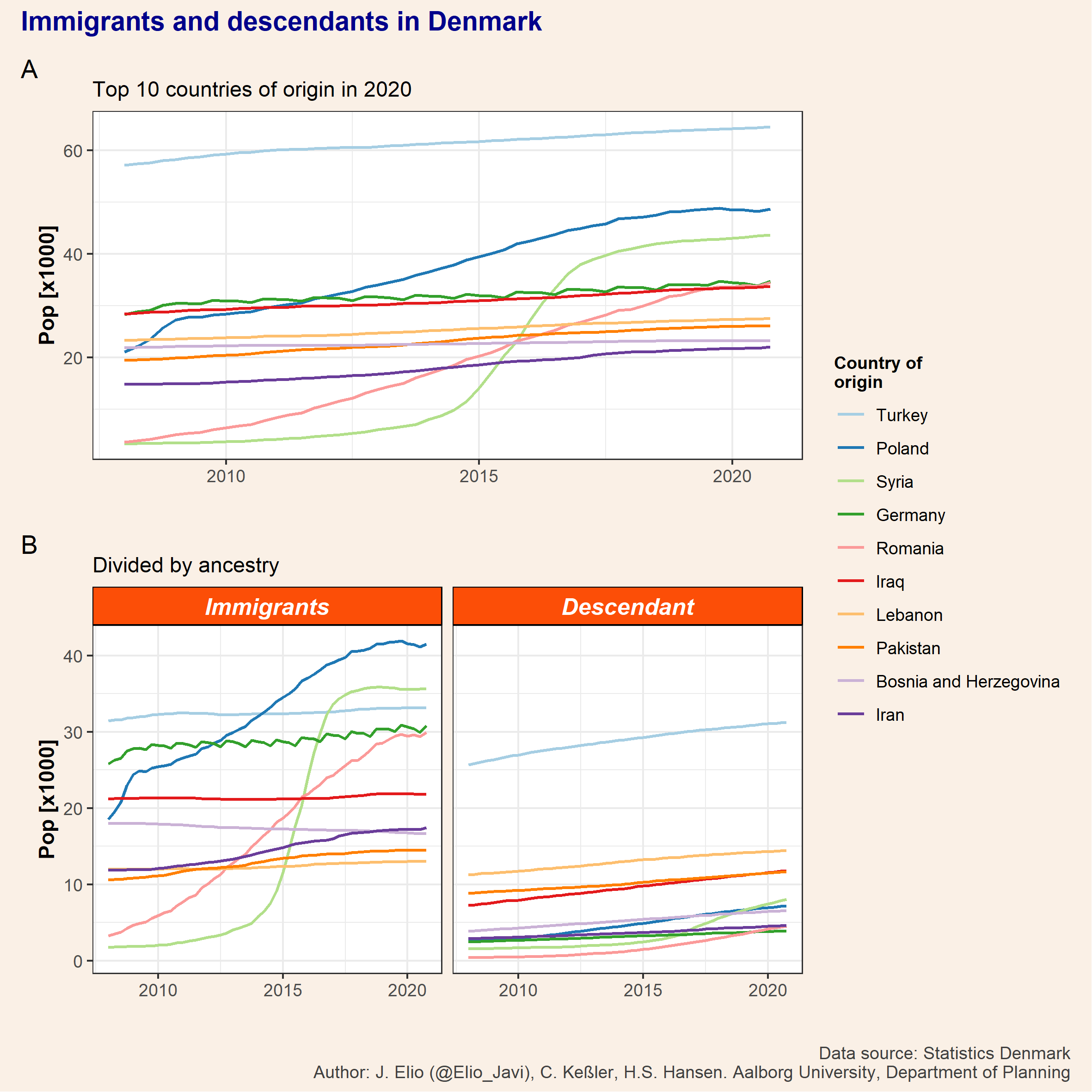
Notes
I have created this post during my work as postdoctoral researcher at Aalborg University, in the project “Global flows of migrants and their impact on north European welfare states - FLOW”.
It is not endorsed by the university or the project, and it is not maintained. All the data I use here are public, and my only aim is that the post serves for learning R. For more information about migration and the project outcomes please visit the project’s website: https://www.flow.aau.dk.
Javier Elío
Associate Professor
My research interests include environmental sciences and data analysis.